AI-Enabled Conflict Simulation
We use Abmarl’s simulation interface to connect a C++ based conflict simulation JCATS to reinforcement learning algorithms in order to train an agent to navigate to a waypoint. All state updates are controlled by the JCATS simulation itself. Positional observations are reported to the RL policy, which in turn issues movement commands to the the simulator. We leveraged Abmarl as a proxy simulation to rapidly find a warm start configuration. Training is performed on a cluster of 4 nodes utilizing RLlib’s client-server architecture. We successfully generated 136 million training steps and trained the agent to navigate the scenario.
JCATS and the PolicyClient Infrastructure
JCATS is the Joint Conflict And Tactical Simulation developed and maintained by Lawrence Livermore National Laboratory. It’s objective is to simulate real conflict in real time with real data. It is a discrete-event, agent-based conflict simulator that can simulate land, air, and sea agents in open scenarios. The user interacts with the simulation through a GUI, from which we can control a single agent all the way up to an entire task force.
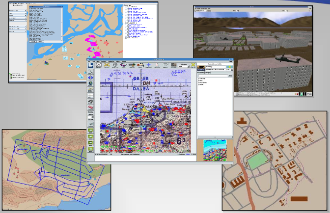
User experience in JCATS, including the GUI and 3d renderings.
JCATS supports two modes: (1) human-interactive mode and (2) batch mode. In the interactive mode, the user interacts with JCATS via a GUI, which provides a graphical visualization of the state of the simulation. We can pause the simulation, query static and dynamic properties of agents and terrain to build up observations, and we can issue actions to the agents in our control. To support human-interaction, the simulation runs throttled: it is artificially slowed down for the user to keep pace with it. While this mode is great for its purpose, it is too slow for reinforcement learning application, which requires the simulation to rapidly generate data.
JCATS batch mode requires pre-scripted plan files made up of action sequences. The simulation runs the actions from those files unthrottled, generating huge amounts of data very quickly. The drawback in batch mode is that we cannot dynamically update the action sequence mid-game, which is necessary for our reinforcement learning interest.
We wanted the speed of batch mode with the dynamic action control of interactive mode, so we leveraged JCATS’s client-server architecture to create a PolicyClient. State and action functions and variable are exposed to a client object, which is wrapped with PyBind11 to bring the functionality to Python. The PolicyClient is a general-purpose interactive interface that can be used to drive JCATS and connect it with other libraries in Python, including open-source reinforcement learning libraries.
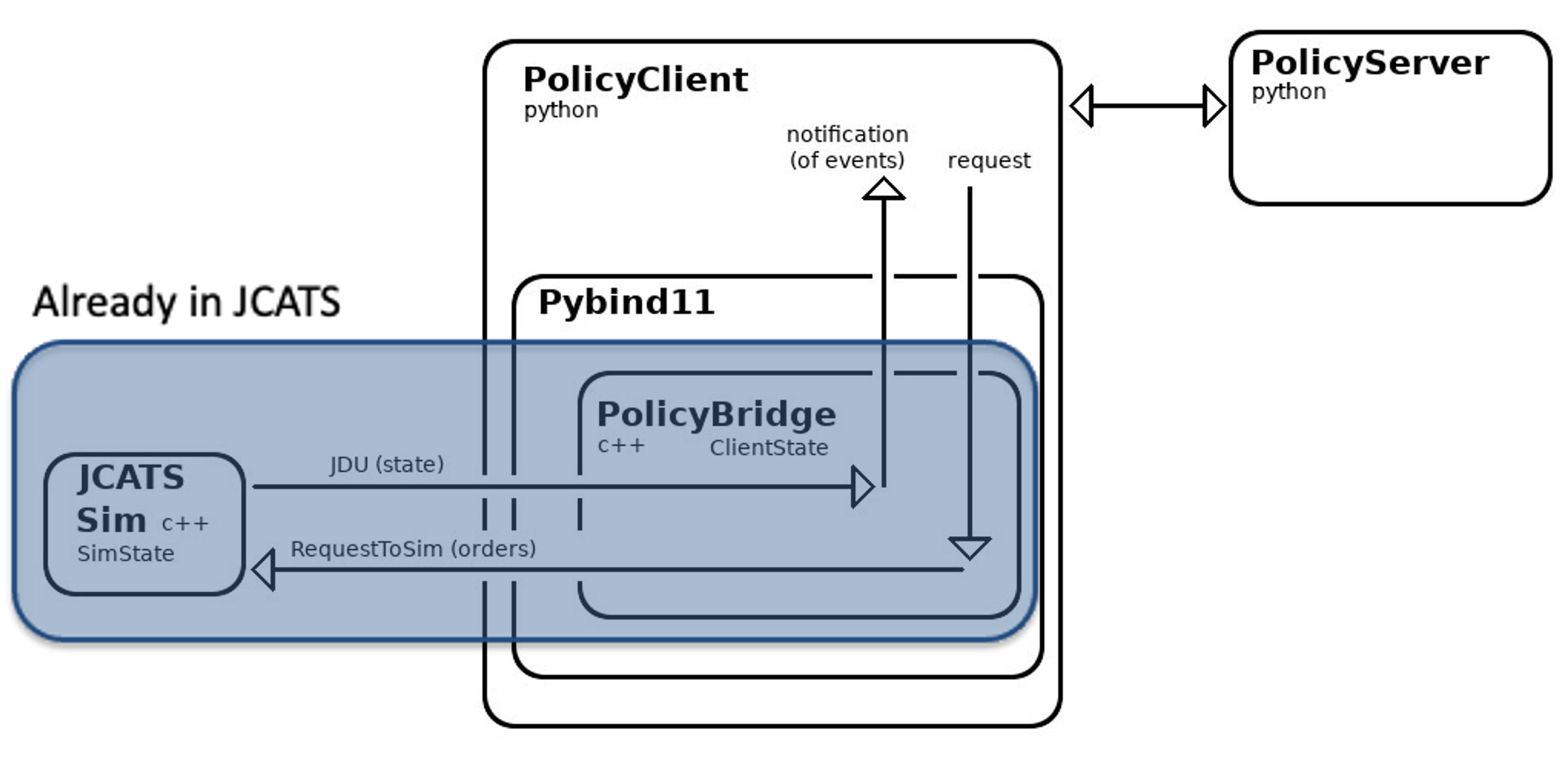
How the PolicyClient fits into JCATS’s client-server architecture.
Scaling Training with RLlib
RLlib is an open-source reinforcement learning libraries written in python. It utilizes a client-server architecture to accomplish reinforcement learning training at scale on HPC systems. The trainer is the server that receives data from the clients, which it processes according to the specific reinforcement learning algorithm to update the policy and send those updated weights to the clients. Each client node has a local instance of JCATS, allowing the node to quickly generate rollout fragments locally. As the rollout fragments build up, the client sends them to the server and receives policy updates asynchronously.
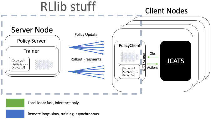
Scalable training with RLlib’s client-server architecture.
We have two dimensions of scalability available to us. First, we can launch multiple instances of JCATS on a single compute node. Second, we an have muliptle client nodes, all connected to the same training server.
JCATS Navigation Scenario
The JCATS Navigation Scenario is set in a continuous spatial domain and contains a set of buildings interconnected with fences, among which there are several paths an agent can take to reach a waypoint. The agent, a single infantry unit, must navigate the 2100x2100 maze by issuing movement commands in the form of continuous relative vectors (up to 100 units away) while only observing its exact position and nothing about its surroundings.

Collection of buildings and fences that make up a maze scenario. The JCATS agent must learn to navigate the maze by issuing local movement commands.
Abmarl Simulation Interface
We wrap the PolicyClient interface with an Abmarl Agent Based Simulation
class to connect the JCATS simulation with RLlib.
The observation space is a two-dimensional continuous array of the agent’s position,
which ranges from (0, 0) to (2100, 2100). The action space is a relative
movement vector that captures the agent’s movement range, from (-100, -100)
to (100, 100).
We need to discretize the time steps in order to use JCATS to generate SAR-tuples like a discrete-time simulator. We determine the minimal amount of time needed for the simulation to process moving our agent 100 units away and set this as the discrete time-gram. Any time less than this and the agent would essentially be wasting some of its action space since the simulation would not process the full state update before requesting another action from the policy. Thus, in each step, the policy will issue a movement command, and then the PolicyClient tells the simulation to run for 50 simulation seconds.
Proxy Simulation with Abmarl’s GridWorld Simulation Framework
We leveraged Abmarl’s GridWorld Simulation Framework to serve as a proxy for the JCATS navigation scenario. The corresponding Abmarl scenario is a 20x20 discrete grid with barriers located in approximately the same locations as the buildings in the JCATS scenario. The agent issues movement commands in the form of discrete relative vectors. Abmarl serves as a particularly good proxy because it can generate data 300x faster than JCATS, enabling us to iterate experiment configuration to answer questions like:
What does the agent need to observe?
How does it need to be rewarded?
What are good hyperparameters for the learning algorithm?
How should we design the neural network?
We can work through learning shots in Abmarl much faster than in JCATS to find a configuration that we can use as a warm-start for the JCATS training.
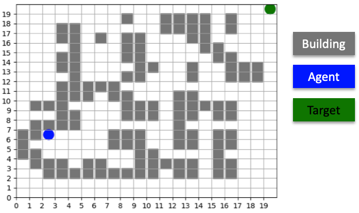
Abmarl proxy scenario, used for finding good training configurations.
Searching for Rewards and Observations
The two most pressing questions are (1) how should the agent be rewarded and (2) what does it need to observe. For the sake of this demonstration, we show three different configurations:
Training Time |
Simulation Steps |
|
|---|---|---|
Regional Awareness |
1 minute |
132 thousand |
Only Position |
30 minutes |
2.5 million |
Position with Soft Reward |
2 minutes |
300 thousand |
Regional Awareness
In this configuration, the agent can observe the surrounding region. It is rewarded for reaching the waypoint on the other side of the grid and penalized for making invalid moves (e.g. moving into a barrier). Training this scenario in Abmarl took one minute and required 132 thousand steps. This is a great configuration, but it is difficult to implement regional-awareness in JCATS because it requires the ability for the PolicyClient to provide a local subset of the simulation state.
Only Position
In this configuration, the agent can only observe its absolute position. It is rewarded for reaching the waypoint and penalized for making invalid moves. This configuration is easy to implement in JCATS because it only requires exposing a single state variable, namely the agent’s absolute position. However, training is difficult because the policy must learn to map absolute position to movement without any knowledge of surroundings. Training this scenario in Abmarl took 30 minutes and required 2.5 million steps.
Soft Reward
In this configuration, the agent only observes its absolute position. It is rewarded for reaching the waypoint, and there are no penalties. This configuration is easy to implement in JCATS and easy to train. Training this scenario in JCATS took two minutes and 300 thousands steps.
A few training runs in the course of less than one hour enabled us to find a good training configuration for the JCATS training shot, thanks to Abmarl’s GridWorld Simulation Framework.
Decision Field Analysis
We query our trained policy over all the cells in our grid to produce a direction field, showing us a visual depiction of the navigation policy. If we imagine the arrows pointing “down” the gradient, we can see that the policy learns to direct all movements to the “valley” which is the shortest path to the waypoint.
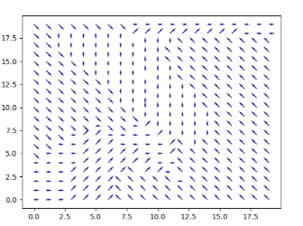
The direction field serves as an tool for analyzing what a policy learns and how its performance evolves over time.
Training and Analysis in JCATS
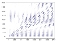
Finally, we take our reward+observation configuration and apply it to JCATS for training on our HPC systems. We utilize RLlib’s client-server architecture to train with 4 client nodes and one server node, with 64 instances of JCATS on each node for a total of 256 data collectors. After one hour of training, we see that the policy begins to move the agent in the correct direction, which is generally to the Northeast.
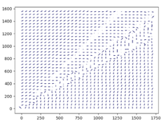
To push our infrastructure even further, we ran the training scenario for 10 days, totalling 61,440 core hours, and successfully generating 136 million training steps without any faults in the duration of training. The direction field shows finer-grained adjustments to the policy to navigate around specific obstructions along the way.
We see in the video below that the agent has learned to navigate the maze of buildings and fences to reach the waypoint.

Agent successfully navigating the JCATS maze to reach the target.
This work was performed under the auspices of the U.S. Department of Energy by Lawrence Livermore National Laboratory under contract DE-AC52-07NA27344. Lawrence Livermore National Security, LLC.
Content has been reformatted from its original presentation LLNL-PRES-851032.