Design
A reinforcement learning experiment in Abmarl contains two interacting components: a Simulation and a Trainer.
The Simulation contains agent(s) who can observe the state (or a substate) of the Simulation and whose actions affect the state of the simulation. The simulation is discrete in time, and at each time step agents can provide actions. The simulation also produces rewards for each agent that the Trainer can use to train optimal behaviors. The Agent-Simulation interaction produces state-action-reward tuples (SARs), which can be collected in rollout fragments and used to optimize agent behaviors.
The Trainer contains policies that map agents’ observations to actions. Policies are one-to-many with agents, meaning that there can be multiple agents using the same policy. Policies may be heuristic (i.e. coded by the researcher) or trainable by the RL algorithm.
In Abmarl, the Simulation and Trainer are specified in a single Python configuration file. Once these components are set up, they are passed as parameters to RLlib’s tune command, which will launch the RLlib application and begin the training process. The training process will save checkpoints to an output directory, from which the user can visualize and analyze results. The following diagram demonstrates this workflow.
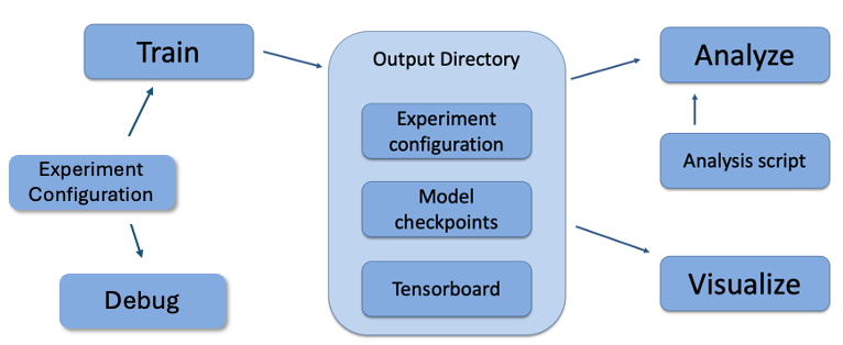
Abmarl’s usage workflow. An experiment configuration is used to train agents’ behaviors. The policies and simulation are saved to an output directory. Behaviors can then be analyzed or visualized from the output directory.
Creating Agents and Simulations
Abmarl provides three interfaces for setting up agent-based simulations.
Agent
First, we have Agents. An agent is an object with an observation and action space. Many practitioners may be accustomed to gym.Env’s interface, which defines the observation and action space for the simulation. However, in heterogeneous multiagent settings, each agent can have different spaces; thus we assign these spaces to the agents and not the simulation.
An agent can be created like so:
from gym.spaces import Discrete
from abmarl.tools import Box
from abmarl.sim import Agent
agent = Agent(
    id='agent0',
    observation_space=Box(-1, 1, (2,)),
    action_space=Discrete(3),
    null_observation=[0, 0],
    null_action=0
)
At this level, the Agent is basically a dataclass. We have left it open for our users to extend its features as they see fit.
In Abmarl, agents who are done will be removed from the RL loop–they will no longer provide actions and no longer report observations and rewards. In some uses cases, such as when using the SuperAgentWrapper or running with OpenSpiel, agents continue in the loop even after they’re done. To keep the training data from becoming contaminated, Abmarl provides the ability to specify a null observation and null action for each agent. These null points will be used in the rare case when a done agent is queried.
Agent Based Simulation
Next, we define an Agent Based Simulation, or ABS for short, with the
ususal reset and step
functions that we are used to seeing in RL simulations. These functions, however, do
not return anything; the state information must be obtained from the getters:
get_obs, get_reward, get_done, get_all_done, and get_info. The getters
take an agent’s id as input and return the respective information from the simulation’s
state. The ABS also contains a dictionary of agents that “live” in the simulation.
An Agent Based Simulation can be created and used like so:
from abmarl.sim import Agent, AgentBasedSimulation
class MySim(AgentBasedSimulation):
    def __init__(self, agents=None, **kwargs):
        self.agents = agents
    ... # Implement the ABS interface

# Create a dictionary of agents
agents = {f'agent{i}': Agent(id=f'agent{i}', ...) for i in range(10)}
# Create the ABS with the agents
sim = MySim(agents=agents)
sim.reset()
# Get the observations
obs = {agent.id: sim.get_obs(agent.id) for agent in agents.values()}
# Take some random actions
sim.step({agent.id: agent.action_space.sample() for agent in agents.values()})
# See the reward for agent3
print(sim.get_reward('agent3'))
Warning
Implementations of AgentBasedSimulation should call finalize at the
end of their __init__. Finalize ensures that all agents are configured and
ready to be used for training.
Note
Instead of treating agents as dataclasses, we could have included the relevant
information in the Agent Based Simulation with various dictionaries. For example,
we could have action_spaces and observation_spaces that
maps agents’ ids to their action spaces and observation spaces, respectively.
In Abmarl, we favor the dataclass approach and use it throughout the package
and documentation.
Simulation Managers
The Agent Based Simulation interface does not specify an ordering for agents’ interactions
with the simulation. This is left open to give our users maximal flexibility. However,
in order to interace with RLlib’s learning library, we provide a Simulation Manager
which specifies the output from reset and step as RLlib expects it. Specifically,
Agents that appear in the output dictionary will provide actions at the next step.
Agents that are done on this step will not provide actions on the next step.
Simulation managers are open-ended requiring only reset and step with output
described above. For convenience, we have provided three managers: Turn Based,
which implements turn-based games; All Step, which has every non-done
agent provide actions at each step; and Dynamic Order,
which allows the simulation to decide the agents’ turns dynamically.
Simluation Managers “wrap” simulations, and they can be used like so:
from abmarl.managers import AllStepManager
from abmarl.sim import AgentBasedSimulation, Agent
class MySim(AgentBasedSimulation):
    ... # Define some simulation

# Instatiate the simulation
sim = MySim(agents=...)
# Wrap the simulation with the simulation manager
sim = AllStepManager(sim)
# Get the observations for all agents
obs = sim.reset()
# Get simulation state for all non-done agents, regardless of which agents
# actually contribute an action.
obs, rewards, dones, infos = sim.step({'agent0': 4, 'agent2': [-1, 1]})
Warning
The Dynamic Order Manager must be used with a Dynamic Order Simulation. This allows the simulation to dynamically choose the agents’ turns, but it also requires the simulation to pay attention to the interface rules. For example, a Dynamic Order Simulation must ensure that at every step there is at least one reported agent who is not done (unless it is the last turn), which the other managers handle automatically.
Wrappers
Agent Based Simulations can be wrapped to modify incoming and outgoing data. Abmarl’s Wrappers are themselves AgentBasedSimulations and provide an additional unwrapped property that cascades through potentially many layers of wrapping to get the original, unwrapped simulation. Abmarl supports several built-in wrappers.
Ravel Discrete Wrapper
The RavelDiscreteWrapper converts observation and action spaces into Discrete spaces and automatically maps data to and from those spaces. It can convert Discrete, MultiBinary, MultiDiscrete, bounded integer Box, and any nesting of these observations and actions into Discrete observations and actions by ravelling their values according to numpy’s ravel_mult_index function. Thus, observations and actions that are represented by (nested) arrays are converted into unique scalars. For example, see how the following nested space is ravelled to a Discrete space:
from gym.spaces import Dict, MultiBinary, MultiDiscrete, Discrete, Tuple
import numpy as np
from abmarl.tools import Box
from abmarl.sim.wrappers.ravel_discrete_wrapper import ravel_space, ravel
my_space = Dict({
    'a': MultiDiscrete([5, 3]),
    'b': MultiBinary(4),
    'c': Box(np.array([[-2, 6, 3],[0, 0, 1]]), np.array([[2, 12, 5],[2, 4, 2]]), dtype=int),
    'd': Dict({
        1: Discrete(3),
        2: Box(1, 3, (2,), int)
    }),
    'e': Tuple((
        MultiDiscrete([4, 1, 5]),
        MultiBinary(2),
        Dict({
            'my_dict': Discrete(11)
        })
    )),
    'f': Discrete(6),
})
point = {
    'a': [3, 1],
    'b': [0, 1, 1, 0],
    'c': np.array([[0, 7, 5],[1, 3, 1]]),
    'd': {1: 2, 2: np.array([1, 3])},
    'e': ([1,0,4], [1, 1], {'my_dict': 5}),
    'f': 1
}
ravel_space(my_space)
>>> Discrete(107775360000)
ravel(my_space, point)
>>> 74748022765
Warning
Some complex spaces have very high dimensionality. The RavelDiscreteWrapper was designed to work with tabular RL algorithms, and may not be the best choice for simulations with such complex spaces. Some RL libraries convert the Discrete space into a one-hot encoding layer, which is not possible for a very high-dimensional space. In these situations, it is better to either rely on the RL library’s own processing or use Abmarl’s FlattenWrapper.
Flatten Wrapper
The FlattenWrapper flattens observation and action spaces into Box spaces and automatically maps data to and from it. The FlattenWrapper attempts to keep the dtype of the resulting Box space as integer if it can; otherwise it will cast up to float. See how the following nested space is flattened:
from gym.spaces import Dict, MultiBinary, MultiDiscrete, Discrete, Tuple
import numpy as np
from abmarl.tools import Box
from abmarl.sim.wrappers.flatten_wrapper import flatten_space, flatten
my_space = Dict({
    'a': MultiDiscrete([5, 3]),
    'b': MultiBinary(4),
    'c': Box(np.array([[-2, 6, 3],[0, 0, 1]]), np.array([[2, 12, 5],[2, 4, 2]]), dtype=int),
    'd': Dict({
        1: Discrete(3),
        2: Box(1, 3, (2,), int)
    }),
    'e': Tuple((
        MultiDiscrete([4, 1, 5]),
        MultiBinary(2),
        Dict({
            'my_dict': Discrete(11)
        })
    )),
    'f': Discrete(6),
})
point = {
    'a': [3, 1],
    'b': [0, 1, 1, 0],
    'c': np.array([[0, 7, 5],[1, 3, 1]]),
    'd': {1: 2, 2: np.array([1, 3])},
    'e': ([1,0,4], [1, 1], {'my_dict': 5}),
    'f': 1
}
flatten_space(my_space)
>>> Box(low=[0, 0, 0, 0, 0, 0, -2, 6, 3, 0, 0, 1, 0, 1, 1, 0, 0, 0, 0, 0, 0, 0],
        high=[4, 2, 1, 1, 1, 1, 2, 12, 5, 2, 4, 2, 2, 3, 3, 3, 0, 4, 1, 1, 10, 5],
        (22,),
        int64) # We maintain the integer type instead of needlessly casting to float.
flatten(my_space, point)
>>> array([3, 1, 0, 1, 1, 0, 0, 7, 5, 1, 3, 1, 2, 1, 3, 1, 0, 4, 1, 1, 5, 1])
Because every subspace has integer type, the resulting Box space has dtype integer.
Warning
Sampling from the flattened space will not produce the same results as sampling from the original space and then flattening. There may be an issue with casting a float to an integer. Furthermore, the distribution of points when sampling is not uniform in the original space, which may skew the learning process. It is best practice to first generate samples using the original space and then to flatten them as needed.
Super Agent Wrapper
The SuperAgentWrapper creates super agents who cover and control multiple agents in the simulation. The super agents concatenate the observation and action spaces of all their covered agents. In addition, the observation space is given a mask channel to indicate which of their covered agents is done. This channel is important because the simulation dynamics change when a covered agent is done but the super agent may still be active. Without this mask, the super agent would experience completely different simulation dynamics for some of its covered agents with no indication as to why.
Unless handled carefully, the super agent will report observations for done covered agents. This may contaminate the training data with an unfair advantage. For example, a dead covered agent should not be able to provide the super agent with useful information. In order to correct this, the user may supply a null observation for an ObservingAgent. When a covered agent is done, the SuperAgentWrapper will try to use its null observation going forward.
A super agent’s reward is the sum of its covered agents’ rewards. This is also a point of concern because the simulation may continue generating rewards or penalties for done agents. Therefore when a covered agent is done, the SuperAgentWrapper will report a reward of zero for done agents so as to not contaminate the reward for the super agent.
Furthermore, super agents may still report actions for covered agents that are done. The SuperAgentWrapper filters out those actions before passing the action dict to the underlying sim.
Finally a super agent is considered done when all of its covered agents are done.
To use the SuperAgentWrapper, simply provide a super_agent_mapping, which maps the super agent’s id to a list of covered agents, like so:
from abmarl.managers import AllStepManager
from abmarl.sim.wrappers import SuperAgentWrapper
from abmarl.examples import TeamBattleSim

AllStepManager(
    SuperAgentWrapper(
        TeamBattleSim.build_sim(
            8, 8,
            ...
        ),
        super_agent_mapping = {
            'red': [agent.id for agent in agents.values() if agent.encoding == 1],
            'blue': [agent.id for agent in agents.values() if agent.encoding == 2],
            'green': [agent.id for agent in agents.values() if agent.encoding == 3],
            'gray': [agent.id for agent in agents.values() if agent.encoding == 4],
        }
    )
)
Check out the Super Agent Team Battle example for more details.
External Integration
Abmarl supports integration with several training libraries through its external wrappers. Each wrapper automatically handles the interaction between the external library and the underlying simulation.
Warning
In order to use external libraries, the corresponding dependencies must be installed. See the installation instructions for more details.
OpenAI Gym
The GymWrapper can be used for simulations with a single learning agent. This wrapper allows integration with OpenAI’s gym.Env class with which many RL practitioners are familiar, and many RL libraries support it. There are no restrictions on the number of entities in the simulation, but there can only be a single learning agent. The observation space and action space is then inferred from that agent. The reset and step functions operate on the values themselves as opposed to a dictionary mapping the agents’ ids to the values.
RLlib MultiAgentEnv
The MultiAgentWrapper can be used for multi-agent simulations and connects with RLlib’s MultiAgentEnv class. This interface is very similar to Abmarl’s Simulation Manager, and the featureset and data format is the same between the two, so the wrapper is mostly boilerplate. It does explictly expose a set agent_ids, an observation space dictionary mapping the agent ids to their observation spaces, and an action space dictionary that does the same.
OpenSpiel Environment
The OpenSpielWrapper enables integration with OpenSpiel. OpenSpiel support turn-based and simultaneous simulations, which Abmarl provides through its TurnBasedManager and AllStepManager. OpenSpiel algorithms interact with the simulation through TimeStep objects, which include the observations, rewards, and step type. Among the observations, it expects a list of legal actions available to each agent. The OpenSpielWrapper converts output from the underlying simulation to the expected format. A TimeStep output typically looks like this:
TimeStpe(
    observations={
        info_state: {agent_id: agent_obs for agent_id in agents},
        legal_actions: {agent_id: agent_legal_actions for agent_id in agents},
        current_player: current_agent_id
    }
    rewards={
        {agent_id: agent_reward for agent_id in agents}
    }
    discounts={
        {agent_id: agent_discout for agent_id in agents}
    }
    step_type=StepType enum
)
Furthermore, OpenSpiel provides actions as a list. The OpenSpielWrapper converts those actions to a dict before forwarding it to the underlying simulation manager.
OpenSpiel does not support the ability for some agents in a simulation to finish before others. The simulation is either ongoing, in which all agents are providing actions, or else it is done for all agents. In contrast, Abmarl allows some agents to be done before others as the simulation progresses. Abmarl expects that done agents will not provide actions. OpenSpiel, however, will always provide actions for all agents. The OpenSpielWrapper removes the actions from agents that are already done before forwarding the action to the underlying simulation manager. Furthermore, OpenSpiel expects every agent to be present in the TimeStep outputs. Normally, Abmarl will not provide output for agents that are done since they have finished generating data in the episode. In order to work with OpenSpiel, the OpenSpielWrapper forces output from all agents at every step, including those already done.
Warning
The OpenSpielWrapper only works with simulations in which the action and observation space of every agent is Discrete. Most simulations will need to be wrapped with the RavelDiscreteWrapper.
Training with an Experiment Configuration
In order to run experiments, we must define a configuration file that specifies Simulation and Trainer parameters. Here is the configuration file from the Corridor tutorial that demonstrates a simple corridor simulation with multiple agents.
# Import the MultiCorridor ABS, a simulation manager, and the multiagent
# wrapper needed to connect to RLlib's trainers
from abmarl.examples import MultiCorridor
from abmarl.managers import TurnBasedManager
from abmarl.external import MultiAgentWrapper

# Create and wrap the simulation
# NOTE: The agents in `MultiCorridor` are all homogeneous, so this simulation
# just creates and stores the agents itself.
sim = MultiAgentWrapper(TurnBasedManager(MultiCorridor()))

# Register the simulation with RLlib
sim_name = "MultiCorridor"
from ray.tune.registry import register_env
register_env(sim_name, lambda sim_config: sim)

# Set up the policies. In this experiment, all agents are homogeneous,
# so we just use a single shared policy.
ref_agent = sim.sim.agents['agent0']
policies = {
    'corridor': (None, ref_agent.observation_space, ref_agent.action_space, {})
}
def policy_mapping_fn(agent_id):
    return 'corridor'

# Experiment parameters
params = {
    'experiment': {
        'title': f'{sim_name}',
        'sim_creator': lambda config=None: sim,
    },
    'ray_tune': {
        'run_or_experiment': 'PG',
        'checkpoint_freq': 50,
        'checkpoint_at_end': True,
        'stop': {
            'episodes_total': 2000,
        },
        'verbose': 2,
        'local_dir': 'output_dir',
        'config': {
            # --- simulation ---
            'disable_env_checking': False,
            'env': sim_name,
            'horizon': 200,
            'env_config': {},
            # --- Multiagent ---
            'multiagent': {
                'policies': policies,
                'policy_mapping_fn': policy_mapping_fn,
                'policies_to_train': [*policies]
            },
            # --- Parallelism ---
            "num_workers": 7,
            "num_envs_per_worker": 1,
        },
    }
}
Warning
The simulation must be a Simulation Manager or an External Wrapper as described above.
Note
This example has num_workers set to 7 for a computer with 8 CPU’s.
You may need to adjust this for your computer to be <cpu count> - 1.
Experiment Parameters
The strucutre of the parameters dictionary is very important. It must have an experiment key which contains both the title of the experiment and the sim_creator function. This function should receive a config and, if appropriate, pass it to the simulation constructor. In the example configuration above, we just return the already-configured simulation. Without the title and simulation creator, Abmarl may not behave as expected.
The experiment parameters also contains information that will be passed directly to RLlib via the ray_tune parameter. See RLlib’s documentation for a list of common configuration parameters.
Command Line
With the configuration file complete, we can utilize the command line interface
to train our agents. We simply type abmarl train rllib_multi_corridor.py, where
rllib_multi_corridor.py
is the name of our configuration file. This will launch
Abmarl, which will process the file and launch RLlib according to the
specified parameters. This particular example should take 1-10 minutes to
train, depending on your compute capabilities. You can view the performance
in real time in tensorboard with tensorboard --logdir <local_dir>/abmarl_results.
Note
By default, the “base” of the output directory is the home directory, and Abmarl will
create the abmarl_results directory there. The base directory can by configured
in the params under ray_tune using the local_dir parameter. This value
can be a full path, like 'local_dir': '/usr/local/scratch', or it can be
a relative path, like 'local_dir': output_dir, where the path is relative
from the directory where Abmarl was launched, not from the configuration file.
If a path is given, the output will be under <local_dir>/abmarl_results.
Debugging
It may be useful to trial run a simulation after setting up a configuration file
to ensure that the simulation mechanics work as expected. Abmarl’s debug command
will run the simulation with random actions
and create an output directory, wherein it will copy the configuration file and
output the observations, actions, rewards, and done conditions for each
step. The data from each episode will be logged to its own file in the output directory,
where the output directory is configured as above.
For example, the command
abmarl debug rllib_multi_corridor.py -n 2 -s 20 --render
will run the MultiCorridor simulation with random actions and output log files to the directory it creates for 2 episodes and a horizon of 20, as well as render each step in each episode.
Check out the debugging example to see how to debug within a python script.
Visualizing
We can visualize the agents’ learned behavior with the visualize command, which
takes as argument the output directory from the training session stored in
~/abmarl_results. For example, the command
abmarl visualize ~/abmarl_results/MultiCorridor-2020-08-25_09-30/ -n 5 --record
will load the experiment (notice that the directory name is the experiment
title from the configuration file appended with a timestamp) and display an animation
of 5 episodes. The --record flag will save the animations as .gif animations in
the training directory.
By default, each episode has a horizon of 200 steps (i.e. it will run for up to
200 steps). It may end earlier depending on the done condition from the simulation.
You can control the horizon with -s or --steps-per-episode when running
the visualize command.
Using the --record flag will not only save the animations, but it will also
play them live. The --record-only flag is useful when you only want to save
the animations, such as if you’re running headless or processing results in batch.
Analyzing
The simulation and trainer can also be loaded into an analysis script for post-processing via the
analyze command. The analysis script must implement the following run function.
Below is an example that can serve as a starting point.
# Load the simulation and the trainer from the experiment as objects
def run(sim, trainer):
    """
    Analyze the behavior of your trained policies using the simulation and trainer
    from your RL experiment.

    Args:
        sim:
            Simulation Manager object from the experiment.
        trainer:
            Trainer that computes actions using the trained policies.
    """
    # Run the simulation with actions chosen from the trained policies
    policy_agent_mapping = trainer.config['multiagent']['policy_mapping_fn']
    for episode in range(100):
        print('Episode: {}'.format(episode))
        obs = sim.reset()
        done = {agent: False for agent in obs}
        while True: # Run until the episode ends
            # Get actions from policies
            joint_action = {}
            for agent_id, agent_obs in obs.items():
                if done[agent_id]: continue # Don't get actions for done agents
                policy_id = policy_agent_mapping(agent_id)
                action = trainer.compute_action(agent_obs, policy_id=policy_id)
                joint_action[agent_id] = action
            # Step the simulation
            obs, reward, done, info = sim.step(joint_action)
            if done['__all__']:
                break
Analysis can then be performed using the command line interface:
abmarl analyze ~/abmarl_results/MultiCorridor-2020-08-25_09-30/ my_analysis_script.py
Python Script
All of Abmarl’s commands can be used directly in a python script instead of relying on the CLI by importing those moodules and running them with the experiment configuration. For example, if we append the following to the configruation file defined above
# parameters defined here ...

from abmarl.debug import debug
from abmarl.train import train
from abmarl.visualize import visualize

print("\n\n\n# --- Debugging --- #\n\n\n")
debug(params) # Debug the simulation with random policies

print("\n\n\n# --- Training --- #\n\n\n")
output_dir = train(params) # Train the policies with RLlib

print("\n\n\n# --- Visualizing --- #\n\n\n")
visualize(params, output_dir) # Visualize the trained policies in the simulation
we can run the file directly with
python3 rllib_multi_corridor.py
which will debug, train, and visualize the setup. See the full workflow example for more details.
Trainer Prototype
Abmarl provide an initial prototype of its own Trainer framework to support in-house algorithm development. Trainers manage the interaction between policies and agents in a simulation. Abmarl currently supports a MultiPolicyTrainer, which allows each agent to have its own policy, and a SinglePolicyTrainer, which allows for a single policy shared among multiple agents. The trainer abstracts the data generation process behind its generate_episode function. The simulation reports an initial observation, which the trainer feeds through its policies according to the policy_mapping_fn. These policies return actions, which the trainer uses to step the simulation forward. Derived trainers overwrite the train function to implement the RL algorithm. For example, a custom trainer would look something like this:
class MyCustomTrainer(SinglePolicyTrainer):
    def train(self, iterations=10, gamma=0.9, **kwargs):
        for _ in range(iterations):
            states, actions, rewards, _ = self.generate_episode(**kwargs)
            self.policy.update(states, actions, rewards)
            # Perform some kind of policy update ^
Abmarl currently supports a Monte Carlo Trainer
and a Debug Trainer, which is used by abmarl debug
command line interface.
Note
Abmarl’s trainer framework is in its early design stages. Stay tuned for more developments.